Introduction
Reading highway signs is not always easy, especially if it is dark or your vision is imperfect. Kline and Fuchs (1993) conducted an experiment to determine what types of signs are easiest to understand at the farthest distance. They compared the distances required for people to recognize text signs, standard symbolic signs, and "improved" symbolic signs (similar to standard ones, but with contours enhanced to promote visibility) of four common highway signs. They also investigated how much age affects the distance at which the sign was recognized.
Synopsis
Abstract
An experiment is described which examines distances required to read text road signs, symbolic road signs, and an “improved” symbolic road sign with enhanced contours.
Data Set
33 variables and 48 cases
Extensions
Sample road signs and a project.
6 Questions
Experimental design, randomization, graphical analysis, difference in means, significance testing, one-sided and two-sided confidence intervals, confounding factors, correlation, regression, residuals.
Basic: Q1-6
Protocol
The sample consisted of three groups of 16 volunteer subjects, 8 men and 8 women per group, divided on the basis of age. Ages in group 1 ranged from 19-35, in group 2 from 37-59, and in group 3 from 61-76. All subjects had at least a high school education and were active, licensed drivers in good health. Participants all met minimum vision requirements. Signs were shown to the subjects on a video monitor set up to imitate the way a person would see the signs while driving a car under daylight conditions. Sign size increased in small increments until the subject was able to describe the sign satisfactorily. The smallest size at which the sign could be clearly described was called the "threshold." At this point the participant was asked to tell what the sign meant.
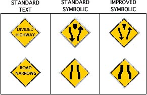
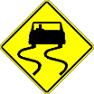
Each participant was shown two series of four signs. The four signs in each series were Divided Highway, Road Narrows, Men Working, and Hill (see examples below). One series contained either the four standard symbolic signs or the improved symbolic signs in random order. The other series contained the corresponding text versions of the four signs, again with the order randomized. In each age group, half of the men and half of the women saw the standard symbolic signs, the other half saw the improved symbolic signs. Whether a participant saw the symbolic signs or the text signs first was also randomized.
Data
The following represents a partial listing of the variables contained in the stored data:
Subject = number assigned to participant
Gender = 1 if male, 2 if female
Age
Age category = 1 if elderly, 2 if middle-aged, 3 if young
Type = 1 if improved symbolic, 2 if standard symbolic
Order = 1 if saw text first then symbolic, 2 if saw symbolic first then text
T-Div High = threshold size of text Divided Highway sign (cm)
T-Rd Nar = threshold size of text Road Narrows sign (cm)
T-Men Wrk = threshold size of text Men Working sign (cm)
T-Hill = threshold size of text Hill sign (cm)
S-Div High = threshold size of symbolic Divided Highway sign (cm)
S-Rd Nar = threshold size of symbolic Road Narrows sign (cm)
S-Men Wrk = threshold size of symbolic Men Working sign (cm)
S-Hill = threshold size of symbolic Hill sign (cm)
DH letter ht = height of the letters on the Divided Highway text sign at the threshold (cm)
RN letter ht = height of the letters on the Road Narrows text sign at the threshold (cm)
MW letter ht = height of the letters on the Men Working text sign at the threshold (cm)
H letter ht = height of the letters on the Hill text sign at the threshold (cm)
Rt. acuity![]() Acuity:The relative ability of the eye to resolve detail. = acuity of right eye (arcmin) (Note: 20/20 vision = 1.0 arcmin)
Acuity:The relative ability of the eye to resolve detail. = acuity of right eye (arcmin) (Note: 20/20 vision = 1.0 arcmin)
Lt. acuity = acuity of left eye (arcmin)
Acuity = best eye acuity (arcmin)
Education = years of schooling completed
WAIS = raw score on the Wechsler Adult Intelligence Scale vocabulary subtest
Vision prob = 1 if vision problems present, 0 if absent
Health prob = 1 if health problems present, 0 if absent
Yrs driving = number of years driving
Questions
Why did the researchers randomize whether a participant saw the text signs or the symbolic signs first?
They randomized the order so that if there happened to be some sort of "learning effect" (i.e. recognizing the second group of signs at a smaller size because you had an idea after the first group what to expect) it would affect both groups and not favor one over the other.
Graphically explore the relationships among the threshold sizes of the three versions of the signs. What do you find?
One option is to make boxplots to compare the threshold sizes of the text signs to the symbolic signs, putting both types of symbolic signs together.
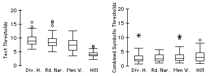
Except for the Hill sign, it appears that the symbolic signs were visible at a much smaller size than the text signs.
One could also compare the two types of symbolic signs to each other.
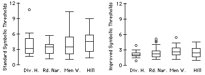
Though the difference between the centers of the two groups is not as striking as between the text and symbolic versions, it does appear that the threshold sizes of the improved signs are smaller than the threshold sizes for the standard symbolic ones. We can also see that there is less variation among the improved thresholds than the standard thresholds.
We are interested in exploring whether the improved symbolic signs are more visible than their standard counterparts.
a) Estimate the mean difference between standard and improved threshold sizes for each of the four types of signs. Write a sentence interpreting what one of these estimates tells us.
b) Kline and Fuchs (1993) used a significance level of 0.01 for all of their inferences. Why do you think they used the more conservative value of 0.01 rather than the common 0.05?
c) Construct a 99% lower confidence bound for the mean difference between standard and improved threshold sizes for each of the four signs. Interpret your results.
d) Why did we construct a one-sided confidence bound in Part c rather than a two-sided confidence interval?
a) If we let ![]() be the observed average standard threshold size and
be the observed average standard threshold size and ![]() be the observed average improved threshold size, then our estimate of the mean difference is
be the observed average improved threshold size, then our estimate of the mean difference is ![]() -
- ![]() .. For the four signs the estimates are:
.. For the four signs the estimates are:
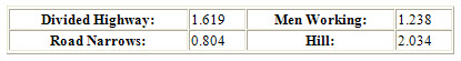
We can say, "On average, the threshold size of the improved Divided Highway sign is 1.619 cm smaller than that of the standard Divided Highway sign."
b) Since it would be very costly to change highway signs if the improved versions are deemed better, the researchers wanted to guard against inappropriately suggesting a change in the current system. They wanted to make sure they had strong evidence before suggesting any possible changes. Therefore they used a significance level of 0.01.
c) We can use the formula (![]() −
− ![]() ) − t
) − t![]()
![]() where
where ![]() =
= ![]() which yields a lower confidence bound for two-sample data, where t is the appropriate cut-off from the t distribution. We can calculate the degrees of freedom for t in two ways, either with Welch's approximation or with min(nx − 1, ny − 1) = 23. (The second method will yield smaller bounds than the first.) The resulting bounds are:
which yields a lower confidence bound for two-sample data, where t is the appropriate cut-off from the t distribution. We can calculate the degrees of freedom for t in two ways, either with Welch's approximation or with min(nx − 1, ny − 1) = 23. (The second method will yield smaller bounds than the first.) The resulting bounds are:
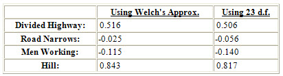
Notice that the bounds for the Road Narrows and Men Working signs are negative. At the 99% confidence level we do not detect a significant difference in threshold sizes for these two signs. For the Divided Highway and Hill signs, however, we are 99% confident that the threshold sizes for the improved symbolic signs are at least 0.516 and 0.843 cm smaller than those for the standard versions respectively.
d) We use a one-sided lower bound because we are only interested in detecting whether the improved signs are significantly better than the standard ones. If the improved and standard signs are equally good or if the data showed the standard signs are better than the improved versions, we would continue to use the standard signs. Only if the improved signs are considered significantly better would we change what we are doing now.
To help us evaluate what practical significance there is in the difference in threshold sizes of, say, a half of a centimeter, we can convert the threshold sizes into another set of units called sight time. Sight time is the time in seconds that a person traveling at 60 mph would have after recognizing a sign until he or she reached the sign. To calculate sight time we use the formula sight time = constant/threshold size. The constant is calculated from the size of the actual road sign, the distance the subject sat from the monitor during the experiment, and the assumed 60 mph speed. The following table gives the average sight times for the three types of signs and the three age groups.
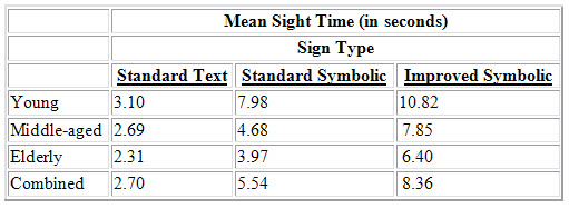
In each age category, people on average would be able to recognize improved symbolic signs about three seconds faster than the standard symbolic counterparts. Do you think that three seconds is enough of a practical significance to justify changing the current road signs? What course of action would you recommend to the highway administration?
The practical significance of three seconds is debatable. On one hand, having eight seconds instead of five to respond may be enough of an improvement to prevent possible accidents. On the other hand, the cost of replacing existing road signs would be prohibitive, and you might argue that five seconds is more than enough time, especially considering text signs only afford three seconds of reaction time. Perhaps you might wish to recommend slowly phasing the new designs into production, and using the improved signs when new signs are needed. It may also be helpful to know the sight times for other speeds such as 50 mph or 35 mph. Information on the average amount of time a driver needs to properly react would be helpful in deciding if three seconds is worth the cost.
a) Consider now the threshold sizes of the text version of the Road Narrows sign. Graphically explore the relationship between a participant's threshold and his or her age.
b) What do you think is causing most of the apparent association between these two variables? If possible, find a variable in the data set that could be a possible confounding factor between threshold and age. One way to do this is to plot possible variables against both threshold and age and see if any are correlated with both. What do you find?
c) Make a scatterplot of the Road Narrows text threshold versus best eye acuity. (Note: a higher acuity measurement indicates poorer vision.) What is the correlation?
d) Instead of the threshold size, suppose we are interested in the size of the letters on the sign when the threshold measurement was taken. Do you think the correlation between the letter size and best eye acuity will be greater than, less than, or equal to the correlation between threshold size and best eye acuity? Why? Verify your guess by computing the correlation.
a) There seems to be a moderate association between threshold size and age, with higher thresholds corresponding to older subjects.
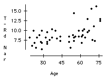
It does appear, however, that the association is not completely linear. The relationship is relatively flat until about age fifty, where there starts to be an increase.
b) When we plot acuity versus both the text threshold and age, we see that both plots show a positive correlation.
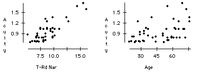
As people age, their eyesight tends to worsen, and people with poor eyesight require larger thresholds to recognize the sign. Thus it does appear that acuity may be a confounding factor between threshold size and age.
c)
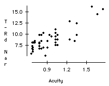
The correlation is 0.810. Higher thresholds correspond to higher acuity levels.
d) We would expect the correlation to be the same. The ratio of letter height to sign height is constant for a particular sign. For any particular subject, if we divide the threshold size of the Road Narrows sign by the letter height threshold we get approximately 8.86. (There is some error due to rounding and measurement error.) Multiplying one of the variables by a constant does not affect the correlation between two variables. The correlation is again 0.810.
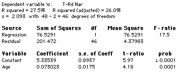
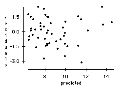
a) Regress the thresholds of the text Road Narrows sign on age. Look at the residual plot. Do you see anything unusual?
b) Try adding acuity to the regression model. Does this variable add anything to the model? Look at a plot of residuals. Do you see anything unusual? Which model do you prefer, the one using age or acuity? Why?
a) The regression output below indicates that age is a significant predictor in this model, but the value of R2 = 27.5% is fairly low. The residual plot below shows no striking pattern.
b) Basic version
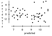
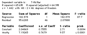
This model looks better than the one using age. The value of R2 = 65.6% is much higher. In other words, 65.6% of variability in T-Rd Nar is explained by the regression on Acuity. The residual plot below for this model shows no obvious problems.
Semi-Tech version
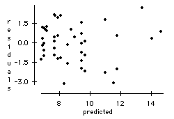
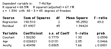
Adding acuity improves the model quite a bit. The value of R2 has increased to 68.5% and the residual plot below shows no obvious problems.
Projects
Design and conduct a similar experiment to determine which of two computer faces can be read from a greater distance. Perform applicable parts of the analysis.
References
Kline, D., and Fuchs, P. (1993)
Credits
This story was initiated by Rebecca Busam and completed by Kathleen Fritsch on 8/25/94. Thanks to Prof. Donald Kline from the Department of Psychology at the University of Calgary for providing the data.