
Introduction
Mercury![]() Mercury:A metallic element highly toxic to the nervous system. It is used in thermometers because of its low melting point. contamination of edible freshwater fish poses a direct threat to human health. This makes it important to know the factors that influence the level of contamination. For example, how does the chemistry of the water in a lake affect the concentration of mercury in the fish that live there? Researchers Lange, Royals and Connor (1993) studied this problem for largemouth bass living in 53 different Florida lakes.
Mercury:A metallic element highly toxic to the nervous system. It is used in thermometers because of its low melting point. contamination of edible freshwater fish poses a direct threat to human health. This makes it important to know the factors that influence the level of contamination. For example, how does the chemistry of the water in a lake affect the concentration of mercury in the fish that live there? Researchers Lange, Royals and Connor (1993) studied this problem for largemouth bass living in 53 different Florida lakes.
Synopsis
Abstract
A study exploring the relationship between lake chemistry and the mercury level in largemouth bass taken from Florida’s lakes is presented.
Data Set
12 variables, 53 cases.
Extensions
Map
8 Questions
Percentages, estimates, standard errors, sample means, regression, transformations, graphical analysis, analysis of residuals, homoscedacity, linear relationships, normality.
Basic: Q1-2, Q5-8
Semi-tech: Q3-4
Protocol
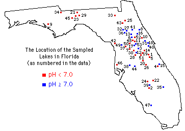
The researchers used their best judgment to choose 53 representative lakes from the 7800 lakes in Florida (see map). Water samples were collected from the surface of the middle of each lake in August 1990 and then again in March 1991. The pH![]() pH:A measure of the degree to which a solution is acidic (smaller numbers) or basic (larger numbers). level, the amount of chlorophyll
pH:A measure of the degree to which a solution is acidic (smaller numbers) or basic (larger numbers). level, the amount of chlorophyll![]() Chlorophyll:The green pigment found in plant cells., calcium, and alkalinity were measured in each sample and then, for each of these variables, the average of the values from the two time points was used in the analysis. Next, a sample of fish was taken from each lake with sample sizes ranging from 4 fish at Parker Lake up to 44 fish at Tohopekaliga Lake. The age and mercury concentration in the muscle tissue of each fish was determined. Since fish will absorb mercury over time, there is a natural tendency for older fish to have higher concentrations of mercury (the typical correlation between age and mercury concentration is about 0.6). Thus, to make a fair comparison of the fish in different lakes, the investigators used a regression estimate of the expected mercury concentration in a three-year-old fish as the standardized value for each lake to be used in the analysis. Finally, in 10 of the 53 lakes, the age of the individual fish could not be determined and the average mercury concentration of the sampled fish was used instead of this standardized value.
Chlorophyll:The green pigment found in plant cells., calcium, and alkalinity were measured in each sample and then, for each of these variables, the average of the values from the two time points was used in the analysis. Next, a sample of fish was taken from each lake with sample sizes ranging from 4 fish at Parker Lake up to 44 fish at Tohopekaliga Lake. The age and mercury concentration in the muscle tissue of each fish was determined. Since fish will absorb mercury over time, there is a natural tendency for older fish to have higher concentrations of mercury (the typical correlation between age and mercury concentration is about 0.6). Thus, to make a fair comparison of the fish in different lakes, the investigators used a regression estimate of the expected mercury concentration in a three-year-old fish as the standardized value for each lake to be used in the analysis. Finally, in 10 of the 53 lakes, the age of the individual fish could not be determined and the average mercury concentration of the sampled fish was used instead of this standardized value.
Data
The following variables are contained in the stored data:
ID number
Lake = name of the lake
Alkalinity (mg/l as Calcium Carbonate)
pH
Calcium (mg/l)
Chlorophyll (mg/l)
Avg Mercury = average mercury concentration (parts per million) in the muscle tissue of the fish sampled from that lake
# samples = how many fish were sampled from the lake
Min = minimum mercury concentration amongst the sampled fish
Max = maximum mercury concentration amongst the sampled fish
3 yr Standard Mercury = regression estimate of the mercury concentration in a three-year-old fish from the lake (or = Avg Mercury when age data was not available)
Age data = 1 if age data is available on sampled fish, 0 otherwise
Questions
The State of Florida has set a standard of 1/2 part per million as the unsafe level of the mercury concentration in edible foods. What percentage of the lakes in this study have standardized mercury concentrations that would be considered unsafe by the state of Florida? Would it be reasonable to use this as an estimate of the percentage of all the lakes in Florida that exceed the declared safety level? Why or why not?
Twenty-four of the 53 (45.3%) lakes in the study had standardized values of at least 1/2 part per million (this includes the 10 lakes for which the ages of the fish were not determined). It is not reasonable to use this as an estimate of the parameter because probability methods were not used to pick the sample. It is also not appropriate to estimate the standard error of the estimated percentage for this judgment sample.
In order to study the accuracy of the technique that was used to analyze mercury concentration, the researchers measured 117 "spiked" fish with a known amount of mercury. The results were an average of 3.9% above the known values with an SD of 9.9%.
Suppose a single fish with a 1 part per million mercury concentration is measured by this method. This measurement is likely to be around ______ give or take ______. Next, suppose this same fish is measured 25 times. The average of these 25 measurements should come out around ______ give or take ______. Fill in the blanks and explain.
The researchers’ study of the quality of their measurement technique shows that it has a bias of about 3.9% and a chance error of about 9.9% of the actual value. A single measurement on a fish with a 1 part per million mercury concentration is likely to come out around 1.039 parts per million give or take about 0.099 parts per million. The average of 25 independent measurements of this same fish should come out around 1.039 parts per million give or take about 0.0198 (= 0.099/251/2) parts per million.
The smallest level of mercury concentration that the measurement technique can detect is 40 parts per billion. Concentrations below this detection limit were reported as 40 parts per billion. How will this affect the standardized mercury concentrations that were used for the final analysis?
For each of the 53 lakes studied, the researchers reported the minimum and maximum mercury concentration found in the sampled fish. Without looking at the data, suggest a function of these two quantities that should have a strong relation with the number of fish taken from the lake. Explain the logic behind your suggestion and then check if it is verified in this data set.
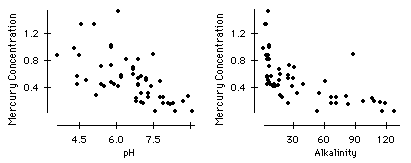
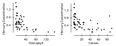
Make scatterplots of the standardized mercury concentration versus the water chemistry variables. Which of the water chemistry variables has the strongest association with the mercury concentration of the fish in the lakes? Which of the associations appear to be linear? Which of the relationships are homoscedastic?
In the plots that follow, alkalinity appears to have the strongest association with the standardized mercury values, although the relationship is non-linear. Only the association with pH appears linear. Only the relationship with alkalinity appears reasonably homoscedastic (particularly on a log scale).
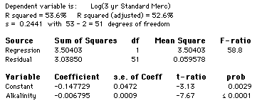
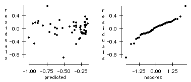
Examine the regression of the logarithm of the standardized mercury concentration on alkalinity.
a) Are the residuals homoscedastic? Do they look like they follow a normal distribution?
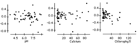
b) Plot the residuals versus the other water chemistry variables. Are there any strong relationships? What does this tell you?
c) Does this regression allow you to say anything about the ages of the fish in the 10 lakes where age wasn't measured?
a) The regression shows that the Alkalinity level of the lake helps to predict the standardized mercury concentration of the fish for the lakes in this study. The residuals are somewhat heteroscedastic with three or four outliers whose residuals are larger in magnitude than would be expected for a normal distribution.
b) The residual plots below indicate the residuals do not appear to be related to the pH or calcium levels in the lakes but there does seem to be a moderate negative association with the chlorophyll level. This tells us that we might improve our prediction of the standardized mercury concentration by including chlorophyll as an explanatory variable in our regression equation.
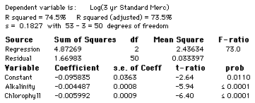
In fact the value of R2 rises from 54% to 75% with the inclusion of chlorophyll. [Note: interestingly, the paper by Lange, Royals, and Connor (1993) found these same two explanatory variables (alkalinity and chlorophyll) as the best two-variable model but did not recognize that using the log of the standardized values gave a superior fit (R2 of 75% instead of 45%).]
c) Yes, some of the variability left in the standardized values for the ten lakes where age was not measured is likely to be due to using the mean mercury concentration instead of the regression-based estimate for a 3 year old fish. Thus, there is likely to be a correlation between the age of the fish in the lakes and the residuals from our best model. It is likely that lake #2 (with the largest positive residual) has older fish than lake #15 (with the smallest negative residual).
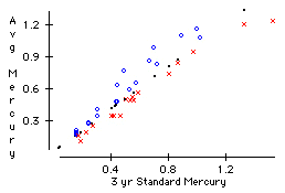
In which lakes was the average age of the sampled fish greater than the three-year-old standard? In which lakes was it less?
Since the correlation between mercury concentration and age is positive, the lakes with a sample average concentration that is larger than the 3 year standard concentration (a regression estimate) must have an average age that is larger than 3 years. Similarly when the sample average concentration is less than the standardized value, the average age must be below 3 years. The ID numbers of the lakes with the older fish (blue o's) are: 6, 7, 8, 9, 14, 18, 19, 20, 21, 26, 27, 31, 35, 36, 40, 43, 44, 45, 49, 51, and 53. The ID numbers of the lakes with the younger fish (red x's) are: 1, 5, 12, 13, 22, 24, 25, 28, 30, 32, 37, 39, 41, 42, 46, 48, and 52.
Researchers Canfield and Hoyer (1988) found that pH and alkalinity generally increase in Florida's lakes as you go from the Northwest to the Southeast and from highland to coastal areas of the state. Does this claim seem to be verified by the 53 lakes (see map below) studied in the article by Lange, Royals and Connor?
The claim seems to be generally true, although this association with geography is not strong.
References
Canfield, D.E., and Hoyer, M.V. (1988)
Lange, T.R., Royals, H.E., and Connor, L.L. (1993)
Credits
This story was prepared by Mike Bowcut and last modified on 5/12/93.