Checkmating and Reading Skills

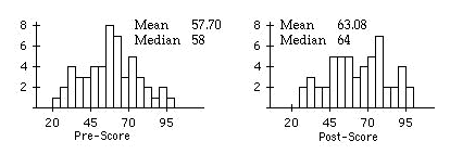
a) Make histograms of the pre-and post-DRP test scores, comment on their shapes, and report both the mean and median for the pre-and post-DRP test scores. Was there an overall improvement in the DRP test scores for the subjects in this study after taking the chess course?

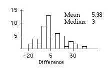
b) Make a new variable of the difference between the post-DRP test scores and the pre-DRP test scores. Calculate appropriate summary statistics for the differences and make a histogram of the data. Do your calculations indicate a general improvement in DRP reading scores for the subjects in this study after receiving the chess instruction? Comment on any interesting features of this histogram. Why is the mean larger than the median for these differences?

• Be able to make (using software where appropriate) and interpret the principle methods of displaying distributions (frequency tables, pie charts, line graphs, bar graphs, and histograms).
• Understand the relationship between key statistical summaries and histograms (for example, mean, median, standard deviation, variance, and quartiles).
• Be able to assess important features of the shape of a distribution by looking at a histogram (single or multiple peaks, symmetric or skewed, the existence of outliers).
• Be able to calculate (using software where appropriate) and interpret the principle measures of center, relative standing, and spread (rates, percentages, mean, median, mode, percentiles, lower quartile, upper quartile, minimum, maximum, standard score, the five-number summary, variance, and standard deviation).
• Understand that the mean and standard deviation are heavily influenced by outliers, whereas the median and the quartiles are not. Because of this, the mean is located farther toward the long tail of a skewed histogram than the median.

a) The means and medians of the post-scores are both larger than the means and medians respectively of the pre-scores. The histograms are both roughly symmetric and show that there were more low scores on the pre-test than on the post-test. The subjects did show an improvement in DRP test scores on the post-test.

b) Both the mean and the median are greater than zero, which indicates that there is an overall improvement in the DRP test scores for the subjects. The histogram also appears to be slightly skewed right. It is this that makes the mean larger than the median. The histogram indicates, however, that not all of the students who took the chess course improved their reading skills.

Make a normal probability plot of the differences between the pre- and post-DRP test scores and comment on any outstanding features of the plot.

• Be able to use a normal quantile plot to assess the normality of a given dataset.
  

The normal probability plot shows that differences between pre- and post-DRP test scores somewhat follow the normal curve. However, the plot also reveals the presence of a slight outlier corresponding to the rightmost bar in the histogram, and again reveals the distribution is skewed right.

a) Was the sample taken in this study a simple random sample? Explain.

b) Give an example of a possible confounding factor in this study, and suggest an appropriate control group which would take this into account.

c) To what population can inference based on the results of this study be made?

• Understand the notion of confounding. Understand how randomization of group assignments yields comparison groups that are similar with respect to confounding factors.

a) It was not a simple random sample. Subjects volunteered to participate in the study. Also, students with DRP scores below the 10th percentile were excluded from the study.

b) It is possible that the students’ reading scores improved because they were getting extra attention from an adult. An appropriate control group might be a similar sample of students who, under the supervision of a teacher, would get together after school to engage in some activity not thought to affect reading, say to listen to classical music.

c) The subjects were not a simple random sample from the population of all grade school students. There is some selection bias in favor of eager students who are willing to give up some time after school in order to participate in the chess instruction. Thus, we should not make conclusions about the effect learning chess will have on all students' reading scores.

a) Use a statistical test on the differences between pre- and post-DRP test scores to test whether there was an improvement in DRP scores after chess instruction. State your hypotheses, report the value of your test statistic, and give the P-value for the test. Provide your conclusions (both statistical and subject matter), and discuss the validity of the assumptions of the test you have chosen.

b) Remove the data point which has a difference between pre- and post-DRP test scores equal to 42 (it is a mild outlier and we wish to see how it affects our results) and repeat the test of Question 4 Part a. State your hypotheses and report the value of your test statistic, the P-value for the test, and your conclusions. Compare your results here to those of Question 4 Part a. Did removing the outlier change your results? Comment.

• Understand the difference between the null and alternative hypotheses. Be able to state the null and alternative hypotheses for a given problem.
• Be able to conduct a formal hypothesis test for a population mean.
• Understand what the components of a hypothesis test are such as: test statistic, alpha level, P-value. Be able to identify these components.
• Understand and be able to check the appropriate distributional conditions underlying the implementation of a significance test (e.g., normal approximation to binomial, chi-square approximation).

a) We wish to test

H₀: Chess instruction does not improve DRP test scores.

versus

H_a: Chess instruction does improve DRP test scores.

Using the one-sample t test we find that t = 3.007 with 52 degrees of freedom. This gives a P-value = 0.002. Thus, we would reject the null hypothesis. There is strong evidence that given a similar sample of students, taking an administered, programmed chess course, we would likely see a rise in the overall average DRP test score of the group.

The result of a one-sample t test is exactly correct only when the population is normally distributed. In Question 2 we found that the data indicated that the population was not normal. However, the t test is robust against non-normality, as the distribution of the sample mean from a large sample is close to normal (central limit theorem) and the sample standard deviation approaches the population standard deviation as the sample size gets large. In this case we have a relatively large sample, so the violation of the normality assumption isn't so serious. A z test is also a reasonable procedure in this case. The t test and z test are not robust against extreme outliers, however, since they are based on the sample mean. Since we only have a mild outlier, we wouldn't expect the results to change too much upon its removal. This is examined in Question 4 Part b. Finally, it would also be reasonable to use a nonparametric procedure such as the sign test here.

b) Again, we wish to test

H₀: Chess instruction does not improve DRP test scores.

versus

H_a: Chess instruction does improve DRP test scores.

Using the one-sample t test we find that t = 2.778 with 51 degrees of freedom. This gives a P-value = 0.0037. Thus, we would reject the null hypothesis. The conclusion of this test is the same as the conclusion of the test done in Question 4 Part a, but the value of t is smaller and the P-value is higher. This is consistent with the fact that the outlier was a maximum and tended to support the alternative hypothesis.

Though the conclusions were the same in this case, one should always be concerned with the presence of outliers when relying upon the results of a t test. The t test is sensitive to outliers because it is based on the sample mean and sample standard deviation, both of which are quite sensitive to outliers. In this case, the relatively large sample size acted to diminish the effect of the outlier.

References

Ferguson, R. (1993)
Margulies, S. (1993)
Credits
This story was prepared by Mark Zabel and last modified on 2/22/95.